©2005-2019 Ulm University, Othmar Marti, released under the
Creative Commons License cc-by-sa 4.0 Lizenzinformationen
[Vorherige Seite] [vorheriges Seitenende] [Seitenende]
[Ebene nach oben] [PDF-Datei][Epub-Datei][Andere
Skripte]
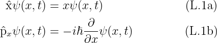
L.1 Kommutator von Ort und Impuls
Wir betrachten zuerst den Orts- ind den Impulsoperator in
der Ortsdarstellung:
Die äquivalenten Definitionen in Mathematica sind
operx := x #1 &;
operpx := - I hbar D[#1,x] &
#1 ist ein Platzhalter, & schliesst die Definition ab. Die
beiden Operationen 
 xψ(x,t) und
  x
x ψ(x,t) werden so
berechnet:
ψ(x,t) werden so
berechnet:
operx[operpx[\[Psi][x]]]
-I hbar x (\[Psi]^\[Prime])[x]
operpx[operx[\[Psi][x]]
-I hbar (\[Psi][x]+x (\[Psi]^\[Prime])[x])
Der Kommutator ist dann
operx[operpx[\[Psi][x]]] - operpx[operx[\[Psi][x]]]
Simplify[%]
-I hbar x (\[Psi]^\[Prime])[x]+I hbar (\[Psi][x]+x (\[Psi]^\[Prime])[x])
I hbar \[Psi][x]
Das ist auch das von Hand ausgerechnete Resultat.
Der Kommutator kann auch als
kommutator := (#1[#2[#3]] - #2[#1[#3]]) &;
definiert werden. Das Resultat ist dann
kommutator[operx, operpx, \[Psi][x]]
Simplify[%]
-I hbar x (\[Psi]^\[Prime])[x]+I hbar (\[Psi][x]+x (\[Psi]^\[Prime])[x])
I hbar \[Psi][x]
[Vorherige Seite] [vorheriges Seitenende] [Seitenanfang]
[Ebene nach oben]
©2005-2019 Ulm University, Othmar
Marti, released under the Creative Commons License cc-by-sa
4.0 Lizenzinformationen